|
How a Photon Is Created or Absorbed
Giles Henderson
Eastern Illinois University, Charleston, IL 61920
Robert C. Rittenhouse
Walla Walla College, College Place, WA 99324
John C. Wright and Jon L. Holmes
University of Wisconsin-Madison, Madison, WI 53706
HTML Translation by Paul Wagner
University of Wisconsin-Madison, Madison, WI 53706
How a Photon is Created or Absorbed is an electronic version of a paper by the same title published in this Journal in 1979 (J. Chem. Educ. 1979 56 631-635). Only minor revisions have been made in the text, but the electronic medium allows interactive graphics and animations that illustrate the points being made much more effectively than could be done in the print medium.
A student typically encounters the concept of a quantum transition in her/his first year of chemistry or physics. A transition is usually depicted as a vertical arrow between two quantum states with emphasis on conservation of energy, i.e., the energy of the photon absorbed or emitted must exactly equal the change in energy experienced by the atom or molecule. At this point, the natural questions of the student are, "How is a photon created or absorbed? What is the mechanism of this process and how long does it take?" The usual instructor response may be that a transition involves a quantum jump which is an instantaneous process and the Uncertainty Principle prohibits us from observing or describing in classical terms the details of the transition, or he/she may evade the question by claiming the concepts are beyond the scope of an introductory course and will be developed later in quantum physics or physical chemistry. After completing a Bachelor degree, our student has been exposed to a lot of the prescriptive formalism of quantum mechanics with heavy emphasis on finding eigenvalues and solutions to the time-independent Schrödinger equation and possibly modest exposure to the time-dependent equation and perturbation theory for the purpose of developing transition probabilities. However, to her/his great disappointment, freshman questions probably still remain unanswered. By now the complexity and abstractness of quantum mechanics has either discouraged pursuit of the answers or convinced her/him that the Uncertainty Principle really does prohibit a conceptual understanding of the process. The stage is set for the cycle to repeat itself for the upcoming generation of students.
The state of affairs has been greatly influenced by over 40 years of popular belief that since a bound system exhibits only certain discrete energies and a transition from one to another cannot proceed through any observable intermediate levels, then the corresponding wavefunction must also evolve in a similar discontinuous manner. This interpretation has been shown to be incorrect (1). To illustrate the problem, consider a two-state system described by the stationary state functions  1(q,t) and 2(q,t) where q and t correspond to the spatial and temporal variables, respectively. Schrödinger (2) interpreted the time-dependent state functions as standing deBroglie matter waves, which are solutions to the differential wave equation 1(q,t) and 2(q,t) where q and t correspond to the spatial and temporal variables, respectively. Schrödinger (2) interpreted the time-dependent state functions as standing deBroglie matter waves, which are solutions to the differential wave equation
 (1) (1)
It is perhaps unfortunate that the time dependence has been highly neglected in the traditional undergraduate texts. This is undoubtedly a consequence of the importance of the eigenvalues and probability function to most problems of interest. Since  1(q) and 2(q) are eigenfunctions of the Hamiltonian (i.e., Hi(q) = Eii(q) the energy eigenvalues are constants of motion and are stationary or invariant in time. The corresponding probability functions are also time independent or stationary since Pi = i*(q,t)i(q,t) = i*(q)i(q). However, it will be shown in this paper that the time dependence of the wavefunction is of crucial importance to understanding the nature of quantum transitions. 1(q) and 2(q) are eigenfunctions of the Hamiltonian (i.e., Hi(q) = Eii(q) the energy eigenvalues are constants of motion and are stationary or invariant in time. The corresponding probability functions are also time independent or stationary since Pi = i*(q,t)i(q,t) = i*(q)i(q). However, it will be shown in this paper that the time dependence of the wavefunction is of crucial importance to understanding the nature of quantum transitions.
If 1 and 2 are of the proper symmetry such that they give a non-zero transition moment integral (3), then electromagnetic radiation, which satisfies the Bohr frequency condition  = (E1-E2)/(h/2 = (E1-E2)/(h/2 ), can stimulate an absorption or emission transition between these states. The formal description of our system during this period of perturbation is given by a linear combination of the stationary state functions sometimes called a superposition function (4): ), can stimulate an absorption or emission transition between these states. The formal description of our system during this period of perturbation is given by a linear combination of the stationary state functions sometimes called a superposition function (4):
 (2) (2)
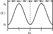
Figure 1. The internal electronic energy of an ensemble of noncolliding atoms subjected to resonance interactions with a monochromatic radiation source. The absorption (ABS) and stimulated emission (EM) process periodically alternates with the Rabi coefficients (eqs (4) and (5)). The period of these alternating cycles,  = (h/2)/( = (h/2)/( < < ij>), is inversely proportional to both the transition moment integral and the intensity of the radiation source. ij>), is inversely proportional to both the transition moment integral and the intensity of the radiation source.
|
where the coefficients c1 and c2 must satisfy the normalization requirement  + +  = 1. Equation (2) describes a nonstationary state that evolves in time and is not an eigenfunction of the Hamiltonian operator. Therefore the energy is not a constant of motion during the transition period. Indeed if an attempt was made to measure the energy during the transition period, the measurement itself would force the system to a stationary state i as a result of the measurement with a probability ci*ci. A common interpretation is that an instantaneous quantum jump in the energy occurred at some unpredictable time during the transition period. This interpretation may in turn suggest that the superposition function is merely a mathematical formalism; if one could observe the evolution of the state, it would also exhibit an abrupt discontinuity or change from i to j or vice versa. The first experimental measurements of bulk samples undergoing spectroscopic transitions were obtained from nuclear magnetic resonance observations of the transient nutation effect (6) and spin echoes (7, 8) using coherent radiation produced by a single radio frequency oscillator. More recently, the analogous transient nutation effect (9, 10) and so called "photon echoes" (11-13) have been observed in molecular spectra using pulsed coherent laser radiation. These experiments confirm that there are no "quantum jumps" in the non-stationary state; rather there are smooth, continuous periodic changes in the magnetic and electric properties of a system undergoing a transition. = 1. Equation (2) describes a nonstationary state that evolves in time and is not an eigenfunction of the Hamiltonian operator. Therefore the energy is not a constant of motion during the transition period. Indeed if an attempt was made to measure the energy during the transition period, the measurement itself would force the system to a stationary state i as a result of the measurement with a probability ci*ci. A common interpretation is that an instantaneous quantum jump in the energy occurred at some unpredictable time during the transition period. This interpretation may in turn suggest that the superposition function is merely a mathematical formalism; if one could observe the evolution of the state, it would also exhibit an abrupt discontinuity or change from i to j or vice versa. The first experimental measurements of bulk samples undergoing spectroscopic transitions were obtained from nuclear magnetic resonance observations of the transient nutation effect (6) and spin echoes (7, 8) using coherent radiation produced by a single radio frequency oscillator. More recently, the analogous transient nutation effect (9, 10) and so called "photon echoes" (11-13) have been observed in molecular spectra using pulsed coherent laser radiation. These experiments confirm that there are no "quantum jumps" in the non-stationary state; rather there are smooth, continuous periodic changes in the magnetic and electric properties of a system undergoing a transition.
In view of these observations it is clear that the superposition function (eq. 2) may be regarded as more than just a formal description; it is indeed real and contains experimentally observable information on the non-stationary, transition species. However, since a superposition function is not an eigenfunction of the Hamiltonian, it is improper to expect that an energy measurement will give an intermediate, time dependent result. The measurement itself will cause the system to change to either its initial or final stationary state with probabilities consistent with and . We can, however, ask for the expectation value of the energy which does change monotonically with time during the transition period (Fig. 1)

 (3) (3)
This result can be interpreted as the energy of an individual atom or molecule at a specified time during its transition period. Of course, neither a single atom nor the energy of an ensemble of transient species can be observed directly. What can be experimentally observed is the distribution of a macroscopic collection of atoms or molecules over the stationary eigenstates. Therefore, a different but equivalent interpretation is that and may be regarded as the probability of observing E1 and E2 from a single measurement of an ensemble of atoms or molecules at a specific time during the transition period. In this study we are concerned with the resonance interaction of uv radiation with frequency ij = (Ej-Ei)/(h/2). Accordingly, the spectroscopic perrturbation to first order will couple only states derivable from i and j. During an absorption transition (i -> j), cj increases at the expense of ci and in the final limit, the excited state is characterized by ci = 0.00 and cj = 1.00. This process is just reversed for emission.
In the case of atoms undergoing absorption or stimulated emission, the coefficents ci and cj have been obtained (5).
 (4) (4)
 (5) (5)
where is electric field strength of the radiation, <ij> is the transition moment integral between the states i and j in the direction of , and t0 is the initial time.
In the limit of large mean free path, low collision frequency,and high electromagnetic field intensities, the dynamics of spectroscopic transitions are dominated by induced absorption and emission processes characterized by eqs. 3-5 above. As collision frequencies increase, or the electromagnetic field intensities decrease, collisional dephasing, spontaneous emission, and radiationless energy transfer begin to compete with the absorption and stimulated emission. Thus, in the typical laboratory measurement where low-power, incoherent sources are used to observe atomic absorption, the non-stationary state is unimportant and optical nutation and other coherent effects are not observed. These effects can be observed in experiments where the radiation source is replaced by an intense laser and the sample is maintained at low pressure or in an atomic beam, effectively eliminating collision-induced processes. Under these circumstances, a laser with a frequency that matches the transition will drive the atoms periodically from their ground state to the excited state as the system absorbs light and from the excited state back to the ground state as the system is stimulated to emit light. The period of this cyclical process is the period of the sinusoidal Rabi coefficients, = (h/2)/(<ij>), as seen in Figure 1. This periodic fluctuation is called transient nutation (6, 9, 10). Experimentally, one observes the laser beam growing alternately dimmer and brighter with a period after it has passed through the collision free atomic sample.
Method
It is now very instructive to examine the time dependence of the non-stationary probability function. From our past experience with quantum mechanics, we can anticipate that a physical understanding of a system is most clearly "seen through the * window" (14). In this case we can expect that * will provide us with a statistical view of the dynamics of nuclear or electronic motion during a transition. David McMillin (15) has recently shown that this approach clearly reveals the origin of an oscillating dipole moment during an electronic transition of a one-electron atom. The probability function is obtained from the superposition wavefunction in the usual manner


 (6) (6)
The first two terms in eq. 6 vary in time directly with the rate of change in and , respectively. However, the last term arises as an interference from the superposition of 1 and 2 and exhibits periodic oscillations at their beat frequency. Since this term is modulated by the product of c1 and c2 the beat amplitudes will systematically build during the beginning of a transition reaching a maximum when  and then decay during the end of the transition period (see Fig. 2). It is this interference term which gives rise to charge oscillations precisely in resonance with the electromagnetic radiation absorbed or emitted during the transition. and then decay during the end of the transition period (see Fig. 2). It is this interference term which gives rise to charge oscillations precisely in resonance with the electromagnetic radiation absorbed or emitted during the transition.
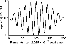
Figure 2. The contribution of the interference term to the dynamic probability function is governed by the product of the time-dependent coefficients. Thus the amplitude of the beat frequency increases during the beginning and decays during the end of the transition period. The time scale given below the figure is only relevant to the discussion of the n=2 <-> n=1 transition in hydrogen (see section Hydrogen Atom in Results and Discussion) and gives the frame number for a 201-frame animation.
|
Three simple model systems will be considered: the rigid rotor, the harmonic oscillator, and the hydrogen atom. In each case dynamic probability functions will be computed for transitions from the respective ground state to the first excited state. For convenience, we will assume a transition period ( t) equal to ten times the period of the electromagnetic radiation (). This is, of course, not realistic for transitions induced by ordinary laboratory source intensities in which t ~ (106-107), but it is obviously impractical to animate 106 oscillations. t) equal to ten times the period of the electromagnetic radiation (). This is, of course, not realistic for transitions induced by ordinary laboratory source intensities in which t ~ (106-107), but it is obviously impractical to animate 106 oscillations.
Results and Discussion
Rigid Rotor
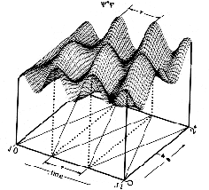
Equation (6) was evaluated for a rigid rotor using normalized spherical harmonic wavefunctions for the states 1 (J = 0, M = 0) and 2 (J = 1, M = 0)
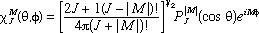 (7) (7)
where  are the associated Legendre Polynomials (16), and the molecular orientation is defined by the angles are the associated Legendre Polynomials (16), and the molecular orientation is defined by the angles  and and  (Fig. 3). Three dimensional computer graphics (17) were used to plot the dynamic probability as a function of the spatial and temporal variables (Fig. 4). For this particular case (M = 0) the functions vary only with and are constant for all values of . On the left side of Figure 4 at time = 0, J = 0, and c2 = 0, the orientational probability (*) is constant for all values of . This result corresponds to the familiar spherical symmetry of the J = 0 state usually depicted as an infinitesimally thin sphere of constant radius and is in accord with the Uncertainty Principle, i.e., in the J= 0 stationary state, the angular momentum is known precisely (L2 = 0), but the spatial orientation or "position" is uncertain (all values of are equally probable). (Fig. 3). Three dimensional computer graphics (17) were used to plot the dynamic probability as a function of the spatial and temporal variables (Fig. 4). For this particular case (M = 0) the functions vary only with and are constant for all values of . On the left side of Figure 4 at time = 0, J = 0, and c2 = 0, the orientational probability (*) is constant for all values of . This result corresponds to the familiar spherical symmetry of the J = 0 state usually depicted as an infinitesimally thin sphere of constant radius and is in accord with the Uncertainty Principle, i.e., in the J= 0 stationary state, the angular momentum is known precisely (L2 = 0), but the spatial orientation or "position" is uncertain (all values of are equally probable).
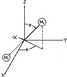
Figure 3. The spatial orientation of a rigid rotor is defined by the conventional spherical polar coordinates, and .
|
During the transition (0 < time < t= and 0 < c2 < 1) the orientational probability surface exhibits two distinct "ridges" which periodically cross the ,time surface. We can imagine a maximum probability (highest elevation) journey across the surface, starting at time = 0 and J = 0 in the left foreground, which, as we advance in time, takes us diagonally across the surface to = 2 in the background. This journey continues from this same point in time from = 2 = 0 in the foreground[1] across the surface again and again until the end of the transition period. We are clearly observing a quantum mechanical, statistically favored trajectory predicting a clockwise rotation (in the direction of increasing ). There is also another exactly symmetrical set of diagonal ridges which cross the surface in the opposite direction describing equally probable counterclockwise rotation. Moreover, the time required for a probability ridge to traverse an angle of = 2 corresponds to precisely the period of the microwave energy, . Thus the analysis confirms a resonance condition in which the frequency of the radiation is exactly equal to the rotational frequency of the rigid rotor. If the rotating molecule possesses a permanent dipole moment there is clearly a mechanism for the oscillating electric field component of the microwave energy to impart a torque on the molecule. The resonance condition will insure a constant phase coherence between the oscillating field and the rotating dipole. The coupling of the external field with the rotating dipole is maximized when their mutual phase angle is /2, since this orientation results in maximum torque. The statistical quantum trajectory can be compared directly with the classical trajectory shown as diagonal lines in the ,time plane directly below the probability surface in Figure 4. The process described above can readily be reversed to describe stimulated emission (J=1 -> J=0). In this case a photon (an electromagnetic wave of finite duration) is "created" at the expense of molecular rotational energy by the periodic rotation of an electric dipole, not unlike radiowaves created by the periodic oscillation of charge in an antenna. The frequency of the radiation is equal to the angular frequency of the rotor. It might also be noted that the radiation will be composed of an equal mixture of right and left circularly polarized components corresponding to equally probable clockwise and counter-clockwise molecular rotations.
Harmonic Oscillator
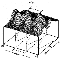
The methods described above can also be applied to the harmonic oscillator. For this case the wavefunctions used in eq. 4 for 1( = 0) and 2( = 1) are = 0) and 2( = 1) are
 (8) (8)
where  is the departure from equilibrium bond length: is the departure from equilibrium bond length:  , ,
 = 42(0)/(h/2), and H() are the Hermite polynomials (18). A plot of the dynamic probability surface for a harmonic oscillator undergoing a transition from =1 <-> =0 is given in Figure 5. In this figure, the surface gives the quantum probabilities of bond lengths as a function of time where q = r-re. On the left side of the diagram, at time = 0, = 0 and c2 = 0, the most probable r is the equilibrium bond length or q = 0. If the system is perturbed by an oscillating electric field of the correct frequency, = [E( = 1)-E( = 0)]/(h/2), then the ground state wavefunction becomes mixed with the excited state function. The resulting time dependent probability function clearly reveals periodic molecular vibrations. A maximum probability (highest elevation) journey takes us periodically back and forth to negative and positive values of q. Indeed, the statistically favored trajectory is an oscillation of bond length at precisely the same period () and frequency (osc = -1) as the infrared radiation. An obvious prerequisite for this resonance interaction is an oscillating molecular dipole. Again we can correlate the quantum trajectory with the classical trajectory shown in the q,time plane of Figure 5. In both the quantum and classical description, the amplitude of the oscillations increases during an absorption transition as the molecule's vibrational energy (or more properly, the expectation value of the molecule's vibrational energy) increases, consistent with the increase in separation of the classical turning points. However, before and after the transition period, the quantum description is very different from the classical description. Classically the molecule continues to oscillate at a fixed amplitude, amplitude = +/-[2E()/k]1/2 and frequency, = (1/2)(k/)1/2 where k and are the force constant and reduced mass of the oscillator, respectively. In contrast, the quantum description of the stationary states gives a time independent probability of bond length and provides no specific details about the dynamics of trajectories. = 42(0)/(h/2), and H() are the Hermite polynomials (18). A plot of the dynamic probability surface for a harmonic oscillator undergoing a transition from =1 <-> =0 is given in Figure 5. In this figure, the surface gives the quantum probabilities of bond lengths as a function of time where q = r-re. On the left side of the diagram, at time = 0, = 0 and c2 = 0, the most probable r is the equilibrium bond length or q = 0. If the system is perturbed by an oscillating electric field of the correct frequency, = [E( = 1)-E( = 0)]/(h/2), then the ground state wavefunction becomes mixed with the excited state function. The resulting time dependent probability function clearly reveals periodic molecular vibrations. A maximum probability (highest elevation) journey takes us periodically back and forth to negative and positive values of q. Indeed, the statistically favored trajectory is an oscillation of bond length at precisely the same period () and frequency (osc = -1) as the infrared radiation. An obvious prerequisite for this resonance interaction is an oscillating molecular dipole. Again we can correlate the quantum trajectory with the classical trajectory shown in the q,time plane of Figure 5. In both the quantum and classical description, the amplitude of the oscillations increases during an absorption transition as the molecule's vibrational energy (or more properly, the expectation value of the molecule's vibrational energy) increases, consistent with the increase in separation of the classical turning points. However, before and after the transition period, the quantum description is very different from the classical description. Classically the molecule continues to oscillate at a fixed amplitude, amplitude = +/-[2E()/k]1/2 and frequency, = (1/2)(k/)1/2 where k and are the force constant and reduced mass of the oscillator, respectively. In contrast, the quantum description of the stationary states gives a time independent probability of bond length and provides no specific details about the dynamics of trajectories.
Hydrogen Atom
The dynamics of the Lyman electronic transition (n=2 <-> n=1) for atomic hydrogen will be considered in this section. If we neglect spin, the stationary state wavefunctions of interest include (19)
 (9) (9)
 (10) (10)
 (11) (11)
where a0 = 0.5292 Å (Bohr radius).
Transitions between these levels are governed by the selection rule l = +/-1 Therefore the transition 2s<->1s is forbidden while the transition 2p<->1s is allowed. The l selection rule can be rationalized on the basis of inversion symmetry considerations (3) or on the basis of conservation of angular momentum (20). The temporal behavior of the superposition function can also provide a useful insight to the origin of the dipole selection rule (15). We will first consider the forbidden 2s<->1s transition. Individual animation frames were obtained by evaluating eq. 6 at 200 regular time intervals corresponding to t = 2.025 x 10⁻¹⁷ sec (Fig. 2). Each frame of the left side animation was produced by encoding the electric charge density in the = /2 (y, z-plane) as a conventional probability dot diagram. Each frame of the right side animation was produced by calculating a rendered isosurface at a selected electron density level using a ray-tracing algorithm.
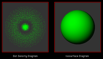
Figure 6. The time evolution of a hydrogen atom undergoing a dipole forbidden (2s -> 1s) transition is animated with a cross section of the charge density encoded as intensity on the left side. The quantum dynamics of the charge density are depicted as a rendered isosurface on the right side. Since the charge density for this process is spherically symmetrical, there is no persistent electric dipole to couple with the surrounding radiation. (Download and play the animation, 1.7 M.)
|
These animations reveal the dynamics of the charge density pulsating at the Bohr frequency, = [E(2s) - E(1s)]/(h/2) with charge "tunneling" back and forth across the 2s nodal surface at r = 2Å. This interesting phenomenon shows the electric charge density in the outer region periodically growing at the expense of the inner charge and then the process reversing. The amplitudes of these oscillations are largest during the middle part of the transition period. The fluctuations in charge are smallest near the beginning and end of the transition period. This merely reflects the magnitude of the product of the coefficients c1c2 of the interference term in the superposition function in eq. 4, (Fig. 2). This animation confirms that although the charge density (and polarizability) is modulated at the correct resonance frequency, there is no oscillating dipole moment in these states. The net charge density is spherically symmetrical for all compositions of the superposition function and therefore there is no mechanism for an external oscillating field to mix these states or to cause this transition by the usual electric dipole interactions. This model indeed confirms the dipole selection rule l ¬ 0 for this transition.
Figure 7 illustrates the dynamics of a transition between the 1s (1,0,0) state and the 2pz (2,1,0) state. During this transition the center of the electron's charge density is periodically displaced in the positive and negative z directions from the nuclear charge giving a persistent oscillating dipole moment. If the process occurs in the direction from 2p->1s under the influence of an external resonance field (stimulated emission) the atom radiates at the Bohr frequency, a "photon" is created. The process is obviously analogous to the production of radio waves by charge oscillating back and forth at the resonance frequency of an r.f. transmitter in a radiating antenna. In the atomic case the oscillation is driven at the expense of the electronic energy of the atom, i.e., the charge density shrinks closer to the nucleus as it dissipates energy. In the direction 2p<-1s the oscillation is driven at the expense of the external field; a "photon" is absorbed. The reader is reminded that these illustrations deliberately distort the duration of the transition period with respect to the period of the oscillation (). Under the influence of ordinary laboratory radiation sources, these transitions would exhibit ~106-107 oscillations during their transition period.
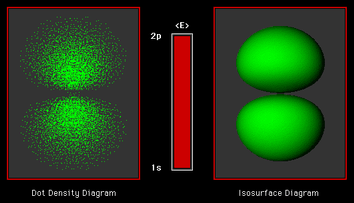
Figure 7. The time evolution of a hydrogen atom undergoing a dipole allowed (2p -> 1s) transition is animated with a cross section of the charge density encoded as intensity on the left side. The quantum dynamics of the charge density are depicted as a rendered isosurface on the right side. These oscillations are driven at the expense of the atom's energy (depicted by the "energy gauge") as the charge density contracts. The atom behaves as a miniature transmitter in which the oscillating electric dipole creates an electromagnetic pulse known as a photon. (Download and play the animation, 1.8 M.)
|
In summary, these methods of illustrating the dynamics of spectroscopic transitions clearly reveal the quantum mechanical origin of oscillating transition moments and the characteristic resonance between the system and the radiation during the creation or absorption of a photon. They provide statistical information on the trajectories of particles which correlate with classical descriptions. The author wishes to express his gratitude to the Eastern Illinois University Council of Faculty Research for financial support of this study.
Literature Cited
- Macomber, J. D., "The Dynamics of Spectroscopic Transition," John Wiley and Sons, N.Y., 1976.
- Schrödinger, E.,Ann. d. Phys., 79, 361, 489; 80, 437; 8l, l09 (1926).
- Kauzmann, W., "Quantum Chemistry," Academic Press, N.Y., 1957, p 661.
- Sherwin, C. W., "Quantum Mechanics," Henry Holt, N.Y., 1959, Chapter 5.
- Rabi I., Phys. Rev. , 51, 652 (1937).
- Torrey, H. C., Phys. Rev., 76, 1059 (1949).
- Hahn, E. L., Phys. Rev., 77, 297 (l950).
- Hahn, E. L., Phys. Rev., 30, 580 (l950).
- Tang, C. L., and Statz, H., Appl. Phys. Lett., 10, 145 (1967).
- Hocker, G. B., and Tang, C. L., Phys. Rev., 184, 356 (1969).
- Kurnit, N. A., Abella, I. D., and Hartmann, S. R., Phys. Rev. Lett., 13, 567 (1964).
- Abella, 1. D., Kurnit , N. A., and Hartmann, S. R., Phys. Rev., 141, 391 (1966).
- Hartmann, S. A., Sci. Amer., 218, 32 (1968).
- Ref. (4), p. 13.
- McMillin, D. R., J. Chem. Educ., 55, 7 (1978).
- Ref. (6), p. 127.
- Watkins, S. L., Communication of the AMC, 17, 520 (1974).
- Ref. (6), p. 77.
- Ref. (4), p. 95.
- Ref. (3), p. 277.
|
|

|